Molecule visualization and initial value problems sample apps

Chemical engineering is a field currently finding itself at the forefront of the energy transition. Single breakthroughs in many chemistry branches concerned with matters like process emission, water pollution or carbon capture could save significant human life and quality of life. In this field, programmers are scarce and thus any working program or piece of codme should be scaled to its ultimate efficacy. VIKTOR can help bring programmers and non-programmers closer together with an easy web app development platform so that progress is developed at a higher speed.

In this article, we present two of such applications developed on the VIKTOR platform. One for the automated generation of basic chemical operations and the corresponding visualizations. The other for the automated visualization of profiles caused by various differential equations.

Sample app molecule visualization

This sample app shows some basic chemical operations and visualizations that are possible in VIKTOR.

Using the functionality

There are two ways in which you can use the functionality:

1. With VIKTOR, out-of-the-box, using our free version

2. Without VIKTOR, in that case you integrate the open-source code with your own Python code.

Below is a snippet of the functionality’s code from app/Chemistry/controller.py:

1@GeometryView('3D', duration_guess=2) 
2def get_3D(self, params, **kwargs): #to make a 3D representation corresponding to a smile 
3	molecule = Chem.MolFromSmiles(params.smile.smile) 
4	molecule = Chem.AddHs(molecule) 
5	AllChem = Chem.MolToMolBlock(molecule) 
6	atoms, atoms_list, bonds = get+positions(block) 
7 
8	geometries = self.make_volumes(atoms, atom_list, bonds) 
9 
10	return GeometryResult(geometries) 

With this function, a smile is made into an RDkit molecule. RDkit finds the most likely position of the atoms. The function handles the reading of positions and bonds, and VIKTOR makes a 3D object out of these.

In the video you can see that the sample app contains an input field for chemical elements, that can be linked to specific properties. It contains another input table for reactants and products that are used to balance reactions. It also has a field for SMILEs, which are strings to represent chemicals, that can be turned into 2D and 3D representations.

Molecule visualization in 3 steps

Visualizing a molecule in VIKTOR can be done in three easy steps:

1. Define input on elements, reactions, and SMILEs. On the right side under the tab ‘Element properties’ you can find the properties of elements from the RDkit library. This shows how VIKTOR cloud display information from databases or internal data sheet.

2. Balance chemical reactions. Under the tab ‘Reaction properties’, you can find information on the balanced reaction based on the input. This shows how simple operations that are complex for non-programmers can be reduced in complexity through interfaces.

3. Visualize SMILES in 2D or 3D (see pictures below). Having visualizations alongside the functionalities that resident programmers can build saves a lot of time clicking back and forth.

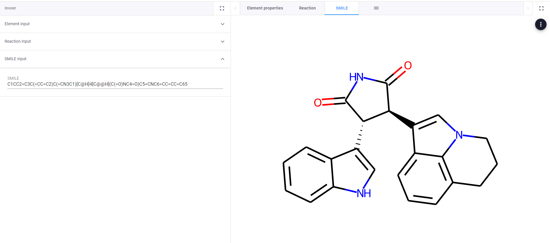
SMILEs visualized in 2D

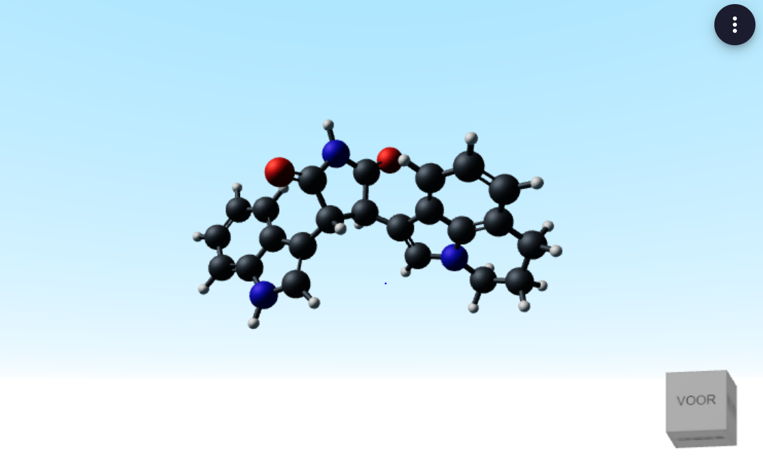
SMILEs visualized in 3D

Sample app initial value problems

This sample app shows how profiles caused by various differential equations are visualized.

Using the functionality

There are two ways in which you can use the functionality:

1. With VIKTOR, out-of-the-box, using our free version

2. Without VIKTOR, in that case you integrate the open-source code with your own Python code.

Below is a snippet of the functionality’s code from app/ODE/controller.py

1def executeODE(self, params): # function for solving the differential profiles based on user input 
2	time = [params.time.begin, params.time.end] 
3	timespan = np.linspace(params.time.begin, params.time.end, params.time.resolution) 
4 
5	initial_conc = get_variable_list(params.species_array.species, ‘concentration’) 
6	applied_reactions = get_variable_list(params.species_array.species, ‘matrix’) 
7	reactions = get_variable_list(params.section_reaction_array.reactions, ‘reaction’) 
8	names = get_variable_dict(params.species_array.species, ‘name’) 
9	constants = get_variable_dict(params.section_reaction_array.reactions, ‘rate_constant’) 
10 
11	names = {name[‘name’]: name[‘index’] for name in names} 
12 
13	sol = solve_ivp(ODEfunx, time, initial_concs, t_eval=timespan, args=[constants, reactions, applied_reactions, names]) 
14 
15	return sol 

Here the table inputs conveniently get made into executable differentials, even though the inputs are strings. The program shows that you don’t have to be a programmer to solve initial value problems with Python when the right infrastructure is in place.

In the video you can see that with the sample app it is easy to simulate profiles of various differentials. The application was originally created to predict chemical reaction profiles, but more applications in which initial value problems require solving can qualify as well.

The sample app contains two tables, one to define the reactions (notation = Reaction: k1AB/k2Bclorine**2, Rate constant: 0.1/0.542) and one to define the species (notation = Name: A/chlorine, Species concentration: 1/3.56, Applicable reactions: -r1+r2/r4-r3+r6*3).

There are also input fields to define reaction time, and plot resolution. Since the program finds and matches strings it can be easy to use abbreviations for the reaction input table. There is one last table where these abbreviations can be subsituted with their full names for the plot legend.

Apply for a demo account to get access to this and all other VIKTOR sample apps.

Initial value problems in X steps

Initial value problems can get complicated quite quickly. You require the changing variables, their initial values, the way their equations change based on all other factors, and the constants for those equations – with chemistry having the added complexity that multiple reactions can influence a species. Luckily, VIKTOR has tables that make this bulky operation as visually digestible as it would be in Excel.

1. In the reaction field, all reactions can be inserted (support multiplication (*), and powers (**)). Users can name species themselves, instead of having to work with Ca and Cb, which can quickly become confusing. All constants k1-kx get a user-defined value.

2. In the species table, all participating species are inserted, with accompanying initial concentrations. In the third column, the reactions that a species undergoes are inserted as well (supports addition (+), subtraction (-), and multiplication (*)), as well as whether it reacts or is formed.

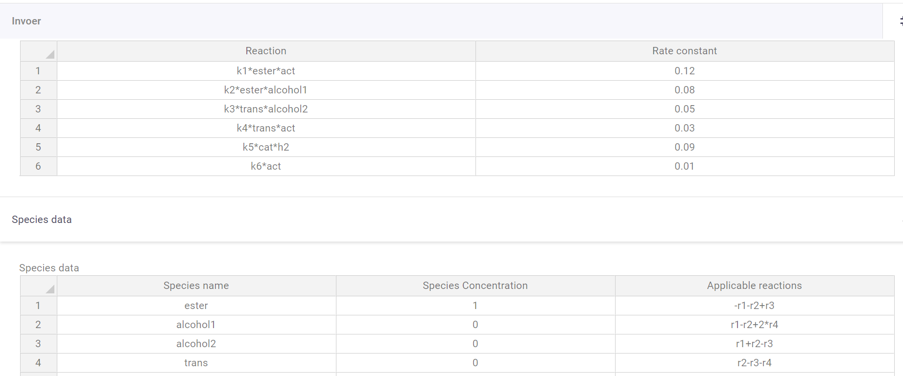
Species table

3. The results from this input yield a graph of the predicted reaction.

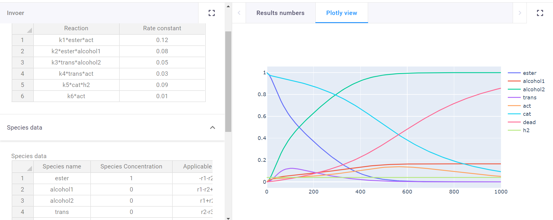
Graph of predicted reaction

Use our free version to start using this app!